I decided to go back to the fundamentals and work up from there. The natural place to start is the basics of neural networks, specifically training them with gradient descent. Interestingly, the mechanism for training neural networks is simple yet powerful for even the most state-of-the-art neural networks.
In this blog post, I try to explain the intuition behind gradient descent, what gradient descent is, what it is used for and how we might go around implementing it from scratch.
The problem
So, before trying to find a solution, we have to understand the problem. Our goal is to somehow learn from given data points and find a somewhat optimal set of parameters that describe the data reasonably well. In other words, our goal is to learn from data points so that it generalizes to unseen data points in the future.
It's easier to understand this with an example. So, let's demonstrate this with linear regression. First, we need our data.
def create_linear_regression_data():
    x = np.arange(0, 10, 1)
    y = x + np.random.normal(0, 1, 10)

    return (x, y)

linear_regression_data = create_linear_regression_data()

plt.scatter(
    linear_regression_data[0],
    linear_regression_data[1],
)
The results from running the code above should look something like the scatter plot below.
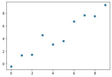 Figure 1. Generated data for linear regression.
The data is generated from the line equation with added Gaussian noise to make it look somewhat random.
Now, we are interested in finding the optimal line that would represent the data points the best. Let's try to do this by hand first.
A line can be represented by two parameters, and , and we need an initial guess for these. Let's say we think and could be somewhat close. We can now plot the line.
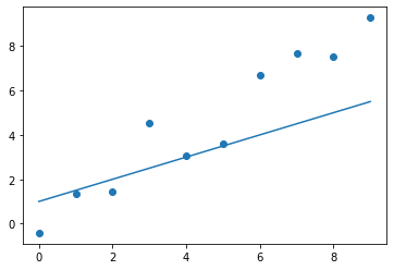 Figure 2. The first guess for the line's parameters.
As we can see, it's not quite there yet, but it's not too far away either. Are we happy with the fit? No. So, we need to tune the parameters in the right direction to get them closer to the optimal values.
The equation of a line is probably quite familiar to all of us, and we have a good understanding of how the parameters affect the line. Therefore, we can intuitively come up with a better guess. Let's say we think that and would yield a better fit.
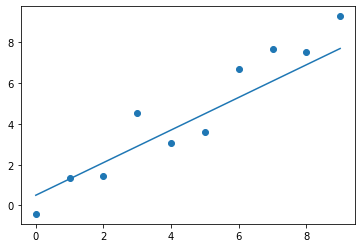 Figure 3. The second guess for the line's parameters.
That's already much better, and it only took us two tries. We could continue to iterate on the parameter values and find an even better fit. But for now, we'll consider this to be good enough for the demonstration.
We used an iterative method for finding the values for the parameters. The technique can be described in four steps.
- Pick somewhat random values for the parameters .
- Visualise how the model fits the data.
- Decide which direction the parameters need to be tuned.
- Tune each parameter a bit and go back to step 2.
These steps are essentially the intuition behind what gradient descent is doing. It looks at the gradients of how different parameters in the model affect the output or loss and tunes the parameters in the direction that makes the model fit the data better. In other words, it tries to descent to the direction where the loss decreases.
There was one critical thing that wasn't entirely clear where it came from. How did we know which direction we needed to tune the parameters to? It was pretty easy in the case of a line, but what if we had 1000s of parameters in our model. In the case of a line, the direction was based on our intuitive understanding of the line equation line, but could we somehow formulate this into a mathematical form?
Gradient descent for linear regression
First of all, what does it mean to have a "good fit" to data? In the case of linear regression, this means that our line passes the data points as close as possible. In other words, we would like to minimize the sum of vertical distances between the predicted line and the given data points.
This combined distance is called the loss function. Its job is to compute the "how bad was the prediction" -metric. We can then use it to calculate the gradient w.r.t. different parameters and tune the model's parameters.
For linear regression, we can use the simple Mean Square Error (MSE) loss function. It is defined as
where is the number of samples, is a target output, and is the predicted output. We are effectively computing the sum of each data point's vertical distance, or residual, to the fitted line.
Our goal is to minimize this loss as that would mean our line is as close to the data points as possible. How do we do that? We compute the gradient of the loss for all parameters.
To be able to compute the gradient, we need to use the chain rule. As a quick reminder, I've written it out below.
Now, let's compute the derivative of the MSE loss w.r.t. .
And now, let's do the same to compute the derivative of the MSE loss w.r.t. .
The result implies that we can compute the gradient of the loss function at any point w.r.t. both parameters of the equation. We should now have some understanding of the gradient part of gradient descent. Let's move to the descent part next.
We can think of the MSE loss function of linear regression as a surface in three-dimensional space. For linear regression, the shape of the loss function is a "bowl."
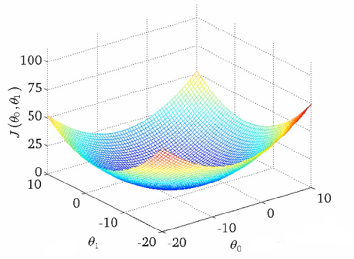 Figure 4. Shape of the MSE loss.
Figure 4 can be found from Towards Data Science's blog post. The shape implies that we can always find the optimal values for the parameters as there is only one global minimum. The only thing we need to do is somehow get to the point where the loss function has the lowest value.
How do we do that? Well, we start at a random point and use the gradient to take steps towards the negative direction of the gradient. This way, we will be moving towards the lowest point of the loss function and eventually find the optimal solution.
To visualize this, let's consider the following simple quadratic function.
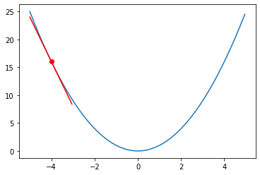 Figure 5. Plot of the quadratic function.
We can pick a single point at and visualized the gradient at that point. Our goal is to optimize the hypothetical parameter to achieve the minimum of the fictional loss function of .
We can do this by computing the gradient at and stepping in the direction of the negative gradient. So, a single step could be something like
where is the learning rate. Take a look at the semi-pseudo-code and the animation below.
alpha = 0.05
z = -4

def do_epoch():
    grad_at_z = 2 * z
    z = z - alpha * grad_at_z

for i in range(50):
    plot()
    do_epoch()
Figure 6. Animation of gradient descent for quadratic function.
We can do the same for linear regression with two parameters. Given the pseudo-code above, we can adapt it to the line equations and apply it to a linear regression problem. The result of doing this can be seen in Figure 7.
 Figure 7. Animation of gradient descent for linear regression.
To summarize gradient descent, I collected the steps required in the list below.
- Define a loss function.
- Compute the gradient of the loss w.r.t. the model's parameters.
- Take a small step in the direction of the negative gradient.
- Go back to step 2 if epochs are left.
Neural networks
Now that we are familiar with the intuition of gradient descent, let's see how we can apply it to neural networks. This section will briefly introduce the topology of our toy-ish neural network, its building blocks and see how we can train them using gradient descent.
Topology of a neural network
In this blog post, we will only focus on fully connected neural networks. There are tons of different variations and architectures that are much more sophisticated than our examples in this blog post. However, even though the training may be more complicated, the fundamental principles are the same. Therefore, we will stick with a simple, fully connected architecture.
A fully connected neural network with two hidden layers might look something like the following.
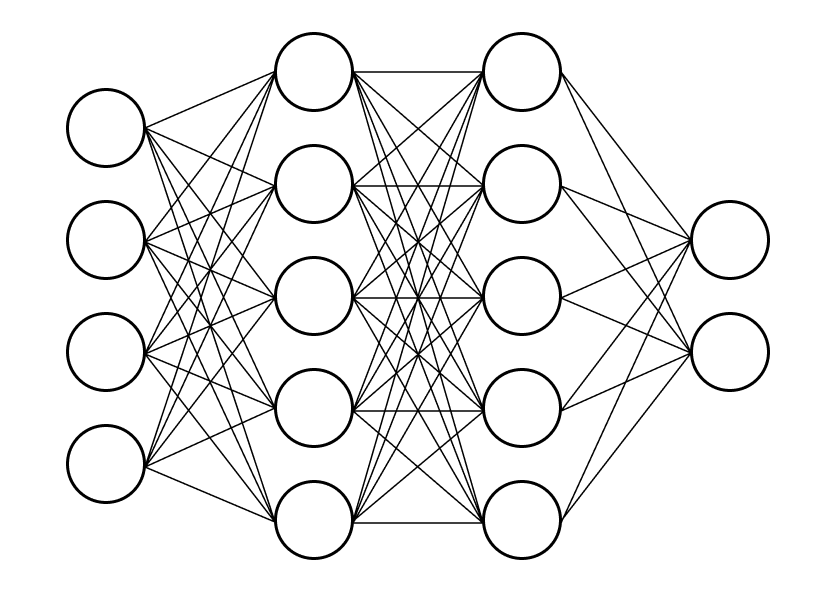 Figure 8. Topology of a fully-connected network.
The left-most layer is the input layer, and the right-most layer is the output layer. In other words, we have 4-dimensional inputs, and we want 2-dimensional outputs, for example, for classification purposes (e.g., cat or dog). The layers in the middle are the hidden layers.
Batch training
Usually, when we train a neural network, we do not pass the entire dataset at once but use multiple batches. This approach is generally called Stochastic Gradient Descent (SGD), where we select a random subset of the samples and use only that subset to make the optimization step.
I'm not going into detail about SGD, but the important part is to understand that we will have samples with features each. We will apply every computation in our neural network to this -by- matrix of input samples.
Note: The math will be written for only a single sample and not a batch of samples. However, our implementation will work on batches.
Building Blocks
This section will zoom in to a single block from Figure 8 and describe what it is composed of. A visualization of a single block can be seen below.
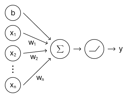 Figure 9. A single block of a fully-connected neural network.
Linear Transformation
The linear transformation is a simple operation that applies a weight to each input and adds a bias term. This operation is similar to what we previously did for the line. However, now we are doing this in -dimensional space instead of 1-dimensional space.
Mathematically, the linear transformation can be formulated as
where is the weight vector and is the bias term. We will need the gradient of the linear transformation for the implementation, so let's calculate those as well.
Implementing the linear layer may look something like the following.
class Linear:
  def __init__(self, in_features, out_features):
    """
    Args:
      in_features  : Number of input features.
      out_features : Number of output features.
    """

    bound = np.sqrt(6 / (in_features + out_features))

    # Initialise the weights and biases
    self.W = np.random.uniform(-bound, bound, (out_features, in_features))
    self.b = np.random.uniform(-bound, bound, (out_features))

    # Internal gradients for learning
    self.dW = None
    self.db = None

  def forward(self, x, W = None, b = None):
    """
    Args:
      x : Inputs of shape (batch_size, in_features).
      W : Optional weights of shape (out_features, in_features).
      b : Optional bias terms of shape (out_features).

    Returns:
      z : Outputs of shape (batch_size, out_features).
    """

    # Decide which weights and biases to use
    _W = self.W if W is None else W
    _b = self.b if b is None else b

    # Keep for gradient
    self.x = x

    return x @ _W.T + _b.T

  def backward(self, dy):
    """
    Args:
      dy : Gradient of the loss w.r.t. 'y'.
           Shape of (batch_size, out_features).

    Returns:
      dx : Gradient of the loss w.r.t. 'x'.
           Shape of (batch_size, in_features).
    """

    # Compute the internal gradients
    self.dW = dy.T @ self.x
    self.db = np.sum(dy.T, axis=1)

    return dy @ self.W
Activation function
The activation function's job is to apply a non-linearity to the output of the node. Multiple possible activation functions are widely used, but we will focus on the simplest one called ReLU.
The proof why we even need an activation function is left out on purpose as it's not relevant to the topic of this blog post. But to summarize, a combination of linear functions is still a linear function. Therefore our neural network would not learn any non-linear functions, making the network entirely unusable.
ReLU is defined as
and its derivative is simply
Implementing ReLU in Python could look something like the following.
class ReLU:
  def forward(self, z):
    """
    Args:
      z : Output from the previous layer.
          Shape of (batch_size, features).

    Returns:
      y : Input after the activation function.
          Shape of (batch_size, features).
    """

    # Note: Keep for gradients
    self.z = z

    return np.maximum(z, np.zeros(z.shape))

  def backward(self, dy):
    """
    Args:
      dy : Gradient of the loss w.r.t. 'y'.
           Shape of (batch_size, features).

    Returns:
      dz : Gradient of the loss w.r.t. 'z'.
           Shape of (batch_size, features).
    """

    return np.where(
      self.z > 0,
      np.ones(self.z.shape),
      np.zeros(self.z.shape)
    ) * dy
Loss function
We will use the same MSE loss as we used previously for linear regression for our toy data.
As a reminder, MSE loss was defined as
and its gradient w.r.t. is defined as
The implementation of MSE loss could look something like the following.
class MSELoss:
  def forward(self, y, target):
    """
    Computes the MSE loss of each entry in the batch.

    Args:
      y      : The actual output from the neural network.
               Shape of (batch_size, out_features).
      target : The target output.
               Shape of (batch_size, out_features).

    Returns:
      c : The loss of each entry in the batch.
          Shape of (batch_size, 1).
    """

    # Note: Keep the differences for the gradient computation
    self.diff = y - target

    return np.sum(np.square(self.diff)) / self.diff.size

  def backward(self):
    """
    Computes the gradient of the loss w.r.t. 'y'.

    Returns:
      dy : The gradient of the loss w.r.t. 'y'.
           Shape of (batch_size, out_features).
    """

    return 2 / self.diff.size * self.diff
Composition
Now that we have the components ready, we need to compose them into a network. We can do this by implementing a new class.
class MLP:
  def __init__(self, name, in_features, hidden_sizes, out_features, activation_fn):
    """
    Args:
      name          : Name of the network.
      in_features   : Number of input features.
      hidden_sizes  : An array of hidden layer sizes.
      out_features  : Number of output features.
      activation_fn : Activation function to use for each layer.
    """

    self.name = name

    # Initialise the first hidden layer
    self.modules = [
      Linear(in_features, hidden_sizes[0]),
      activation_fn()
    ]

    # Initialise the rest of the hidden layers
    for i in range(len(hidden_sizes) - 1):
      self.modules.append(Linear(hidden_sizes[i], hidden_sizes[i + 1]))
      self.modules.append(activation_fn())

    # Initialise the output layer
    self.modules.append(Linear(hidden_sizes[-1], out_features))

  def forward(self, x):
    """
    Do the forward pass.

    Args:
      x : Inputs of shape (batch_size, in_features).

    Returns:
      y : Outputs of shape (batch_size, out_features).
    """

    y = x

    for layer in self.modules:
      y = layer.forward(y)

    return y

  def backward(self, dy):
    """
    Do the backward pass.

    Args:
      dy : Gradient of the loss w.r.t. 'y'.
           Shape of (batch_size, out_features).

    Returns:
      dx : Gradient of the loss w.r.t. 'x'.
           Shape of (batch_size, in_features).
    """

    dx = dy

    for i in range(len(self.modules) - 1, -1, -1):
      dx = self.modules[i].backward(dx)

    return dx
Training
Remember the chain rule I mentioned before? Great, that's going to be very useful now. Let's start with a single block in our neural network. After combining the linear and activation function steps from above, it is defined as
The chain rule stated that we can split the derivative into two separate steps and multiply them by each other. Let's see how that works in our case.
We now have a way to calculate the derivative of a single block's output w.r.t. its inputs in our neural network. However, we are really interested in computing the loss function's derivative w.r.t. the inputs of the entire network.
This is where the chain rule comes in the second time. The network can be represented as nested functions that can use the chain rule to compute the gradient.
The gradient can then be computed in the following way.
Using the chain rule enables us to implement each layer as an independent block that will receive the gradient of the loss w.r.t. the layer's output and will produce the gradient of the loss w.r.t. the layer's input.
In practice, the training progresses in three phases:
- Forward pass, where we pass a batch of inputs through the network.
- Backward pass, where we propagate the gradient from the output to the input.
- Optimization step where we tweak the parameters based on the gradients.
Let's write the code for this.
def generate_toy_data(n, plot = False):
  # First, let's generate a random set of x values
  x = np.sort(np.random.randn(n, 1), axis=0)

  # Let's compute the targets (with Gaussian noise)
  targets = np.sin(x * np.pi / 2) + 0.3 * np.random.randn(n, 1)

  if plot:
    plt.scatter(x, targets, s=10)

  return x, targets

def train_toy_network(activation_fn, epochs = 250):
  # Define our data
  x, targets = generate_toy_data(128)

  # Define parameters for training
  learning_rate = 0.075

  # Define our network and loss
  net = MLP("toy", 1, [20, 20], 1, activation_fn)
  loss = MSELoss()

  # Define the outputs after each epoch
  outputs = np.ndarray((epochs, x.size))

  for i in range(epochs):
    # Forward pass
    y = net.forward(x)
    c = loss.forward(y, targets)

    # Backward pass
    dy = loss.backward()
    dx = net.backward(dy)

    # Gradient descent update
    learning_rate *= 0.998

    for module in net.modules:
      if hasattr(module, 'W'):
        module.W = module.W - module.dW * learning_rate
        module.b = module.b - module.db * learning_rate

    # Append the outputs
    outputs[i, :] = net.forward(x).flatten()

  return (x, targets), net, outputs
How does this look for our toy data? I trained the network with both ReLU and Tanh activation functions for the toy data set, and the results look like the following.
 Figure 10. Animation of gradient descent with ReLU.
 Figure 11. Animation of gradient descent with Tanh.
It's interesting to see what the activation functions are doing here. With ReLU, we get a non-linear function, but it seems to be composed of lines. This makes sense as ReLU's output is either the identity function or cuts off the output completely. On the other hand, Tanh seems much smoother, and it fits our sinusoidal data better.